Add your promotional text...

Mathematics Portfolio
Showcasing my work in mathematics and academic contributions.


Differential calculus is a branch of calculus that focuses on rates of change and slopes of curves. It revolves around the concept of the derivative, which measures how a function changes as its input changes.
At its core, the derivative of a function f(x) at a point x is defined as the limit:
f′(x) = lim(h→0) [f(x+h)−f(x)] / h
This formula represents the slope of the tangent line to the curve y = f(x) at x, capturing how fast f(x) is increasing or decreasing.
Key rules in differential calculus include:
Power Rule: d/dx (x^n) = n x^(n−1)
Product Rule: (fg)′ = f′ g + f g′
Quotient Rule: (fg)′ = (f′ g−f g′) / g^2
Chain Rule: (f(g(x)))′ = f′ (g(x)) g′(x)
Derivatives have vast applications, from physics (velocity and acceleration) to economics (marginal cost/revenue) and engineering (optimization problems). By studying how functions change, differential calculus provides powerful tools for modeling and solving real-world problems efficiently.
Integral calculus is a branch of calculus that focuses on accumulation and area. It is primarily concerned with finding integrals, which are the reverse of derivatives. Integrals come in two main types: indefinite and definite.
Indefinite Integral: This represents a family of functions whose derivative is the given function. It is written as:
∫ f(x) dx = F(x) + C
where F(x) is the antiderivative of f(x), and C is an arbitrary constant.
Definite Integral: This calculates the net area under a curve between two points aa and bb. It is given by:
∫ (a to b) f(x) dx = F(b) − F(a)
according to the Fundamental Theorem of Calculus, which links differentiation and integration.
Integral calculus has many applications, including computing areas under curves, volumes of solids, total accumulated quantities, and solving differential equations. Methods of integration include substitution, integration by parts, and partial fractions.
In essence, while derivatives measure change, integrals measure accumulation.
Calculus with Analytic Geometry integrates the principles of calculus—limits, derivatives, and integrals—with the coordinate geometry of curves and surfaces. This combination allows for a deeper understanding of functions, motion, and optimization in a graphical and algebraic manner.
Key Concepts:
Limits & Continuity – The foundation of calculus, describing how functions behave near specific points.
Derivatives – Measure instantaneous rates of change and slopes of curves, with applications in motion, optimization, and physics.
Integrals – Represent accumulation and area under curves, used in calculating volumes, work, and probabilities.
Coordinate Geometry – Describes curves (e.g., lines, parabolas, circles) using equations, facilitating their study via calculus.
Conic Sections – Parabolas, ellipses, and hyperbolas analyzed using calculus to determine properties like tangents and areas.
By merging calculus with geometry, we can analyze complex shapes, optimize real-world problems, and study motion in space.


Dr. Jamal Teymouri on the right
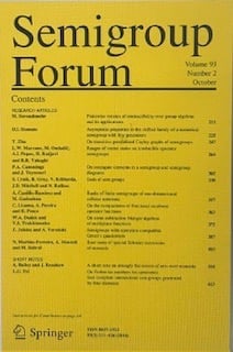
Dr. Teymouri's article on Semigroup Forum